Most thermal modelling projects in automotive spend the majority of their time not solving physics - but configuring it. Setting up geometry representations, mapping cell sensor signals to Simulink ports, assigning material properties, wiring the cooling boundary conditions from CFD into the thermal solver. The same steps, repeated for every new battery variant, every new pack geometry, every new cooling configuration.
The Battery Thermal Model Configurator was built to eliminate that overhead - and to produce something better than what the manual process was generating.
The Problem It Was Solving
At Mercedes-Benz R&D India, the battery thermal modelling workflow involved building coupled Simulink thermal models for high-voltage battery packs. These models had to:
- Represent the thermal mass and conductance of cells, modules, and pack structure accurately
- Incorporate cooling channel behaviour derived from full CFD simulations
- Be directly compatible with the electrical model and the ageing model in the broader simulation framework
- Be audit-ready - traceable, versioned, documentable
Each model took significant engineering time. The cell geometry changes, the module layout changes, the cooling strategy changes - and each change propagated through the entire model setup manually. The process didn’t scale.
The Configurator was the answer.
What Is a Reduced-Order Model?
Before getting into the tool, it helps to understand the problem it sits inside.
A full physics-based thermal model of a battery pack might have millions of degrees of freedom - every point in space has a temperature, every cell has a detailed geometry. Solving that is slow. Running it across thousands of scenarios is impractical.
A Reduced Order Model (ROM) compresses that complexity. It finds a lower-dimensional representation that captures the essential thermal behaviour without resolving every detail.
Think of it like summarising a thousand-page book into a ten-page summary. The fine details are lost. But the plot, the key events, and the critical relationships remain. The reader gets the essence without the time commitment.
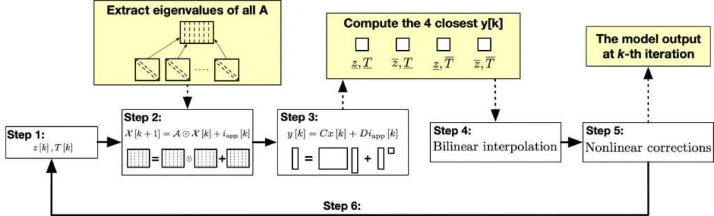
In thermal modelling, a ROM represents temperature distribution using a handful of basis functions and lumped nodes instead of millions of grid points. Accuracy drops a few percent. Speed increases by orders of magnitude. For system-level simulation - where you need to run thousands of scenarios, not compute a single high-fidelity result - that is the right trade-off.
The problem is that building a good ROM is not trivial. The parameters have to come from somewhere. And that is where the Configurator comes in.
The Other Piece: Cooling Plate CFD
A battery pack is not just cells. It has a cooling system - typically an aluminium plate with machined channels. Coolant flows through the channels. Heat transfers from the cells to the coolant.
CFD analysis of the cooling plate gives you the spatially-resolved picture: velocity field inside every channel, pressure drop from inlet to outlet, and the local Heat Transfer Coefficient (HTC) across the plate surface.
The HTC is the key number. It tells you how effectively heat moves from cell surface to coolant. A high HTC means good cooling. A low HTC means the heat stays in the cell and builds up.
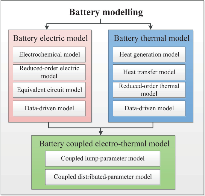
CFD analysis is expensive. Running it for every design iteration isn’t feasible. But running it once - for a baseline design - and then coupling those results intelligently into a fast ROM is exactly the right approach. That coupling is what the Configurator handles.
What It Actually Does
The Configurator operates as a model generation pipeline - taking structured inputs about the battery geometry, cooling configuration, and cell data, and producing a fully parameterised, coupled Simulink thermal model as output.
Reduced-Order Thermal Model of the Battery
Rather than resolving full 3D heat transfer (expensive, slow), the tool builds a lumped thermal network: each cell, module wall, and pack structure is a node with thermal mass, and conductance paths connect them based on geometry and contact properties.
The parameters - thermal resistance between cell and cooling plate, between module and pack wall, effective heat capacity of each node - are not assumed. They are computed from geometry and material data using standardised methods implemented inside the Configurator. Generic, formula-driven HTC and thermal property calculations replace what was previously manual lookup and entry.
CFD Coupling for Cooling Channels
The CFD results - flow distribution, local HTC, coolant temperature rise along the channel - are read by the Configurator and mapped as boundary conditions into the thermal ROM. This is the coupling that makes the model high-fidelity despite being reduced-order. The cell thermal behaviour is lumped; the cooling channel behaviour is physics-derived from CFD. The two are connected at the cooling plate interface.
CFD Simulation Results
(flow distribution, HTC, ΔT_coolant)
           │
           ▼
  Cooling Boundary Conditions
           │
           ▼
┌──────────────────────────────────┐
│     Lumped Thermal Network       │
│  Cell → Module → Pack Structure  │
│  (thermal mass + conductances)   │
└──────────────────────────────────┘
           │
           ▼
  Coupled Simulink Thermal Model
  (compatible with electrical + ageing models)
Sensor Location Recommendation
Thermal sensors cannot be placed everywhere - cost, wiring, and packaging constraints limit instrumentation. The Configurator analyses the HTC variation across the cooling plate and recommends optimal sensor placement: one sensor near the outlet (highest temperature, lowest HTC), one near the inlet (lowest temperature), covering the gradient the BMS actually needs to manage.
This is not just a convenience feature. Getting sensor placement wrong means the BMS is either flying blind in the hot spot, or wasting channels on redundant cool-zone measurements. The recommendation is grounded in the CFD-derived HTC map, not engineering guess.
Signal Mapping: Sensors and Simulink Ports
A battery pack has cell-level temperature sensors at defined physical locations. The simulation model needs to output signals at those same locations - so that BMS logic and the validation process work against consistent sensor positions.
The Configurator handles automatic mapping of cell sensor signals to Simulink output ports, and input/output port mapping for the full model interface. At scale (hundreds of cells in a large HV pack), manual port mapping is a genuine source of bugs. This eliminates that class of error.
Pressure Calculations
Coolant flow requires a pump. The pump consumes energy. That energy comes from the battery itself.
A poorly designed cooling plate has high pressure drop - the pump works harder, and the net system efficiency drops. The Configurator calculates coolant pressure drop from the CFD results and passes it to the system model, so the energy cost of cooling is accounted for in the overall vehicle energy budget. A small but important coupling that is often missed in simplified thermal-only models.
Power Loss Architecture
One of the enhancements implemented was a structured power loss hierarchy - from cell-level Joule heating (I²R), through module-level aggregation, to pack-level totals. This replaced a simpler assumption of uniform heat generation and improved model accuracy, particularly for high-rate discharge and fast charging scenarios where cell-to-cell current distribution is uneven.
A Practical Example
Suppose a battery pack for an electric vehicle. The thermal engineer designs a cooling plate with a serpentine channel pattern. A CFD analysis shows hot spots near the outlet, where the coolant has already warmed up. The HTC is 20% lower there compared to the inlet.
The Configurator takes this data. It maps the HTC variation to the cell positions above the cooling plate. Cells near the outlet get lower HTC. Cells near the inlet get higher HTC. The thermal ROM reflects this spatial non-uniformity automatically.
Sensor recommendation: place a temperature sensor near the outlet cells - that is the hot spot. The BMS uses this reading to limit power when temperatures rise.
Pressure drop calculation: 5 kPa at nominal flow rate. The Configurator passes this to the system model, which calculates that the pump will consume approximately 50 W. That load is subtracted from usable pack energy in the system-level simulation.
All of this happens in a single automated run. No manual scripting. No guesswork. A documented, reproducible output - audit-ready from the first run.
Outcomes
| Metric | Result |
|---|---|
| Model development time reduction | 60% |
| Workflow standardisation | Consistent process across all pack variants |
| Manual preprocessing errors | Significantly reduced |
| Model compatibility | Direct integration with electrical + ageing models |
| Audit traceability | Every parameter has a documented source |
The 60% reduction came from a combination of: automated HTC and property calculations, automatic signal mapping, and the structured generation process replacing ad-hoc manual assembly.
What Made This Hard
The CFD-to-ROM interface. CFD gives spatially-resolved results; the ROM needs boundary conditions at specific nodes. The mapping requires decisions about how to aggregate distributed heat transfer coefficients into representative lumped values without losing the information that actually matters - local hot spots, flow maldistribution effects. Getting this wrong produces a model that looks reasonable on nominal cases and fails on edge cases.
Sensor mapping at scale. A large HV battery pack can have hundreds of cells and tens of temperature sensors. Getting the Simulink port structure right - and keeping it traceable to the physical sensor layout - required careful architecture of the mapping logic.
Keeping it audit-ready. Internal toolchain at Mercedes-Benz R&D had to pass review. The Configurator output had to be traceable: every parameter, every boundary condition, every mapping had to have a documented source. Building that traceability into the generation process, rather than as a manual annotation step afterwards, was a design constraint that shaped the architecture.
Why This Matters Beyond the Project
The Configurator is an example of a recurring pattern in simulation-heavy engineering: the meta-problem - the problem of building the infrastructure that makes the actual problems faster to solve - is often worth more engineering investment than another incremental improvement to the solver.
A 60% reduction in model development time, compounded across multiple battery programmes and multiple years, is a larger return than almost any accuracy improvement to the model itself. The constraint wasn’t model fidelity. It was throughput.
That instinct - identify where the time actually goes, then engineer a solution to that - has appeared in every subsequent role.