Most battery models fail not because the equations are wrong - but because the assumptions smuggled in with them are wrong.
Fifteen years working with battery models across the stack: from ECM spreadsheets that needed to survive a BMS real-time loop, to full electrochemical models trying to capture what actually happens inside the cell during a fast charge. The gap between “runs on paper” and “works in a vehicle” is where most of the interesting problems live.
This isn’t a single project - it’s the accumulated understanding from building, validating, and deploying battery models across multiple OEMs, chemistries, and applications. The failures taught more than the successes.
The Three Ways to Model a Battery
Equivalent Circuit Model (ECM)
An RC circuit that impersonates a battery. A voltage source, a series resistance, and one or more RC pairs representing diffusion dynamics. Fast, tunable, works in real-time on a BMS microcontroller.
The issue isn’t that it’s inaccurate - for a narrow operating window, it’s fine. The issue is that you don’t know when it breaks. Push the cell outside the temperature or SoC range you calibrated on, and the model degrades silently. There’s no physics to signal the extrapolation; it just drifts.
The real trap is over-tuning. More RC pairs → better fit on characterisation data → worse generalisation. A 3-RC ECM that fits HPPC data beautifully can fail badly predicting a 2C discharge from a warm start - because the additional poles absorbed noise in the training data, not real dynamics.
ECM earns its place in: BMS applications, real-time SoC estimation, anything requiring sub-millisecond compute time, early-stage pack design where a fast model is needed before full characterisation data exists.
ECM Structure (1-RC example):

V_terminal = OCV(SoC) - I·R₀ - V_RC

where V_RC evolves as: dV_RC/dt = I/C₁ - V_RC/(R₁·C₁)

R₀, R₁, C₁ - all functions of temperature and SoC
OCV - measured from slow discharge (quasi-static)
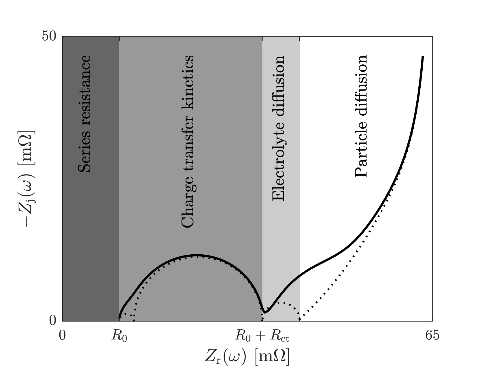
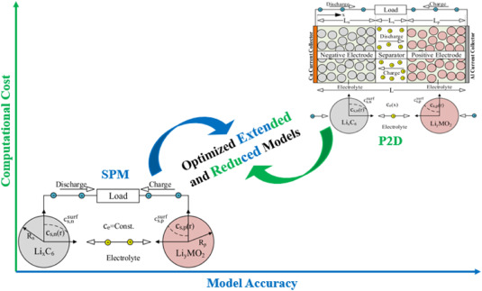
Electrochemical Model (DFN / P2D)
This is the actual physics. Doyle-Fuller-Newman (DFN) or its single-particle simplification (SPM): Butler-Volmer electrode kinetics, Fickian diffusion of lithium in solid particles and through the electrolyte, Nernst-Planck ion transport, conservation of charge and mass across both electrodes and separator.
The model knows why the voltage drops - not just that it does. It can tell you that the voltage sag at high C-rate is diffusion-limited at the cathode, not kinetics-limited at the anode. That distinction matters for aging prediction and for designing fast-charge protocols.
The catch is parameterisation. A full DFN model has 20–30 parameters, most of which you cannot measure directly. Solid-phase diffusivity, exchange current density, electrolyte transference number - these require careful experimental protocols and parameter estimation from indirect measurements. Get the diffusivity wrong, and your model predicts lithium plating onset at the wrong SoC. That’s not a small error - that’s the wrong safety boundary.
DFN earns its place in: Understanding aging mechanisms, designing fast-charge limits, studying capacity fade, anything where you need to ask why the cell behaves as it does.
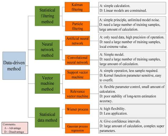
Data-Driven / Stochastic Model
A Hidden Markov Model, a neural network, or a Gaussian process treats the battery as a system to be learned from data rather than derived from first principles. No physics equations - just patterns extracted from measurements.
It’s honest in a way the ECM isn’t: it doesn’t claim to know the physics. The problem is the same as all black-box models - it’s a compression of the training distribution. Show it an operating condition outside that distribution and you get smooth, confident nonsense. No warning lights, no physical plausibility check.
Data-driven earns its place in: Short-horizon prediction under controlled and well-characterised operating conditions, health estimation when abundant historical data exists, anywhere the physics is genuinely unknown or too complex to parametrise.
The Tradeoff That Structures Everything
All three model classes trade off along the same axes:
| ECM | DFN / P2D | Data-Driven | |
|---|---|---|---|
| Physical interpretability | Low | High | None |
| Computational cost | Very low | High | Variable |
| Extrapolation range | Poor | Good | Very poor |
| Parameterisation effort | Low | High | Data-hungry |
| Aging mechanism visibility | None | Full | Indirect |
The instinct is to pick one and defend it. The right answer is almost always a hybrid - use the electrochemical model to build physical intuition and identify dominant mechanisms, then encode that structure into a fast surrogate.
The ECM’s RC parameters aren’t arbitrary numbers - they correspond to something physical. R₀ is predominantly ionic resistance in the electrolyte and contact resistance. The RC pair time constants correspond to diffusion timescales in the electrode particles. You can derive their temperature and SoC dependence from electrochemical first principles instead of fitting them empirically to characterisation data. The result is an ECM that extrapolates correctly - because its parameters have physical backing, not just curve-fit backing.
That’s the direction that actually scales across applications and operating conditions.
Where Models Break (and What That Teaches You)
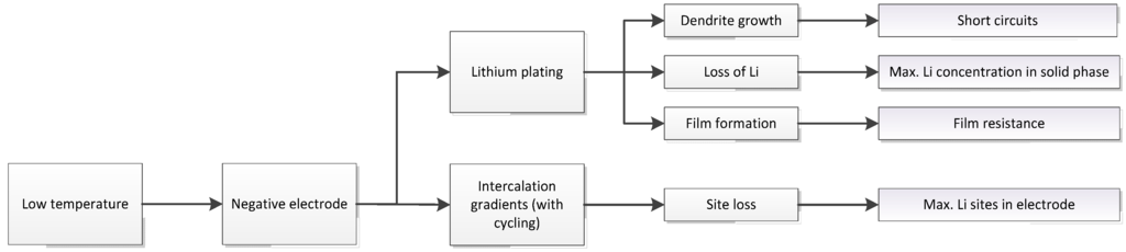
Cold temperatures. Lithium diffusion in graphite has Arrhenius temperature dependence - halve the temperature (in Kelvin) and diffusivity drops by orders of magnitude. An ECM calibrated at 25°C will underestimate voltage sag at -10°C and overestimate available power. A DFN model will capture this correctly if the diffusivity parameters are identified from low-temperature data.
End of life. As the cell ages, internal resistance increases, active material decreases, and the OCV curve shifts. An ECM recalibrated from fresh-cell data will predict the wrong SoC for an aged cell. This is why SoH-adaptive parameterisation is not optional for a BMS that needs to work across the vehicle’s life.
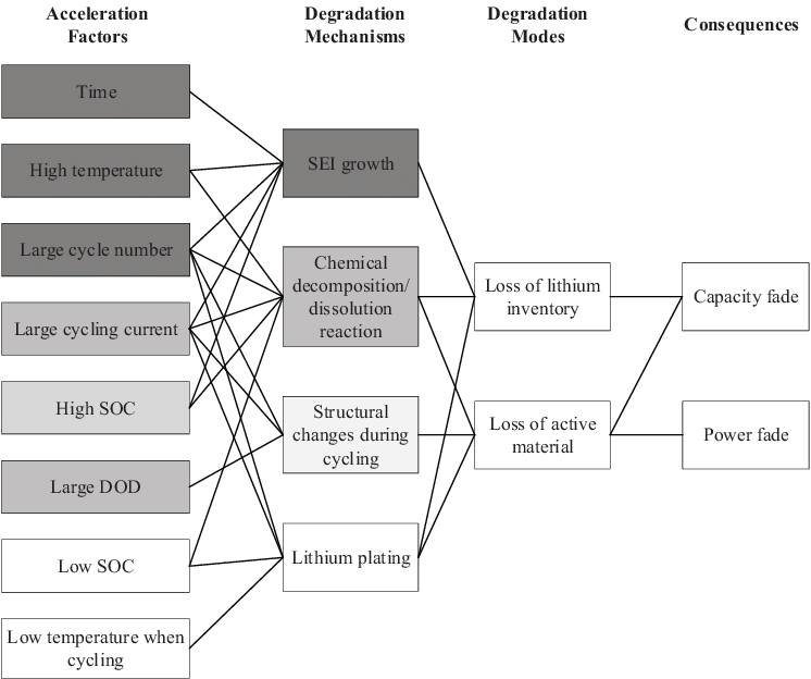
Fast charge. The interesting physics during fast charging is at the anode - diffusion limitation causes anode potential to drop toward 0V vs Li/Li⁺, and if the charging current is too high, lithium plates rather than intercalates. An ECM cannot detect this. A DFN model can, because it tracks anode potential explicitly.
First cycles. The SEI layer forms in the first few cycles, consuming lithium inventory and setting the baseline internal resistance. Models calibrated after formation but applied to predict formation losses will be systematically wrong.
What I’m Still Working Through
- How to reliably detect lithium plating onset in real-time from terminal measurements alone - without computational budget that rules it out for BMS deployment
- How aging mechanisms interact and couple: SEI growth slows diffusion, which shifts the plating boundary, which changes the operating limits, which affects SEI growth rate. The nonlinear coupling across timescales (seconds to years) is genuinely hard
- Whether physics-informed neural networks can bridge the gap between interpretability and computational cost - or whether they just add complexity without adding understanding
How This Connects to the Broader Work
Battery models don’t live in isolation. They feed:
- BMS state estimation - SoC, SoH, power limits
- Thermal management - heat generation is a model output, not a measurement
- Aging prediction - calendar and cycle life, capacity fade trajectories
- Fast-charge protocol design - the limits on charge rate come from the electrochemistry, not from conservative engineering judgment
The interesting problems aren’t at 25°C and 50% SoC. They’re at cold start, at the end of a fast charge, at end of life, at the boundary conditions where model quality actually determines whether the system works correctly or fails safely.